Quick Start Guide
This page aims to take you though fitting your first set of data in FSL-MRS. This web-based guide is now supplemented with a dedicated MRS section in the online FSL Course.
FSL Course
The FSL Course now contains a dedicated section on MRS. This includes three videos on:
and an online written practical. Data for the practical is available by following the online instructions.
Online Guide
Below we describe an end-to-end pipeline that includes data conversion, processing, model fitting, quantification, and visualisation of the results. To apply this step to the example data provided with FSL-MRS see the example_usage section in the main package.
1. Convert your data
Before running FSL-MRS, time domain data must be prepared in a complex NIfTI-MRS format. You can do this by running the accompanying spec2nii tool (see Data Conversion).
Example conversion:
spec2nii dicom -f my_metab_file metab.dcm
This will convert the dicom file (metab.dcm) to a NIfTI file named my_metab_file.nii.gz. Conversion of other formats is possible by changing the first argument “dicom” to another option. For a list of supported formats see Data Conversion.
A directory of DICOM data can also be converted:
spec2nii dicom -f my_metab_file ./dcm_metab_dir/
The output of the above command will also be my_metab_file.nii.gz but the converter will append dynamics into higher NIfTI-MRS dimensions (continuing up to the number of DICOM instances in the directory).
You might need to covert multiple files to process a single spectroscopy acquisition. A typical single voxel dataset will have both water suppressed and water unsuppressed data. Depending on format these might be contained in a single raw data file or be spread over two or more. Some protocols may acquire additional data to be used in pre-processing, e.g. for eddy-current correction. These files should be converted with a different name:
spec2nii dicom -f my_wref_file ./dcm_wref_dir/
spec2nii dicom -f my_ecc_file ./dcm_ecc_dir/
But note that there are frequently multiple calibration scans for e.g. shimming and water suppression calibration acquired before the actual MRS acquisition. These files aren’t used for analysis and can be safely ignored.
1.1 Take a look at your data
You can use mrs_tools info and mrs_tools vis on the command line to view your data at any stage of the process. First mrs_tools info to see the dimensionality of the data:
mrs_tools info my_metab_file.nii.gz

Read file my_metab_file.nii.gz (/path_to_file).
NIfTI-MRS version 0.2
Data shape (1, 1, 1, 4096, 32, 64)
Dimension tags: ['DIM_COIL', 'DIM_DYN', None]
Spectrometer Frequency: 297.219948 MHz
Dwelltime (Bandwidth): 8.330E-05s (12005 Hz)
Nucleus: 1H
Field Strength: 6.98 T
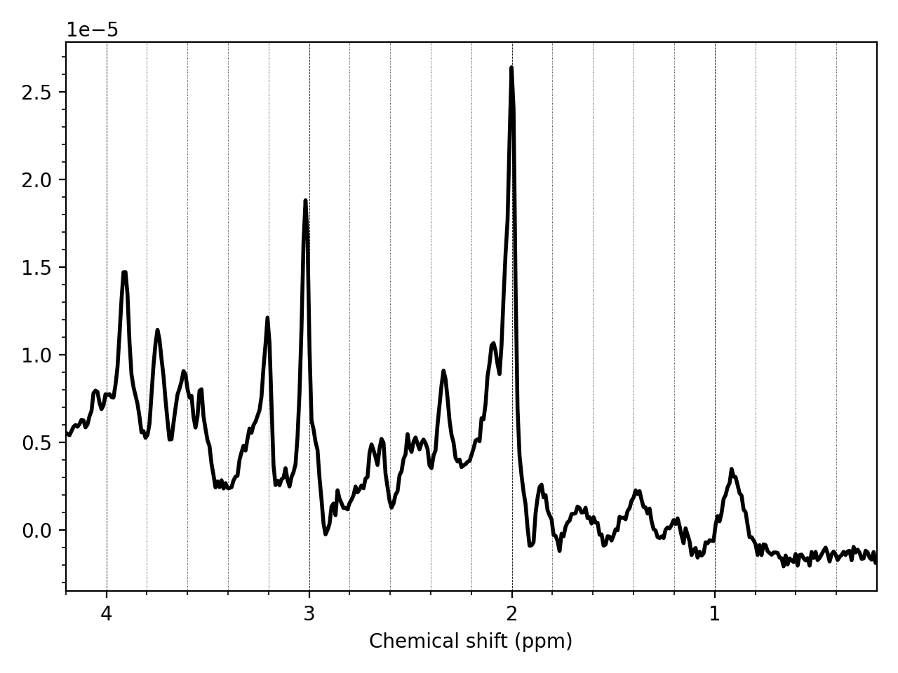
Then mrs_tools vis to visualise the data:
mrs_tools vis my_metab_file.nii.gz
mrs_tools vis will automatically perform coil combination and averaging down to a single spectrum for display purposes only.
You can also quickly view data across one of the NIfTI-MRS higher dimensions (those containing uncombined coils, or averages etc.) In this case we plot all the transients stored in the dimension tagged DIM_DYN (i.e. averages):
mrs_tools vis my_metab_file.nii.gz --display_dim DIM_DYN
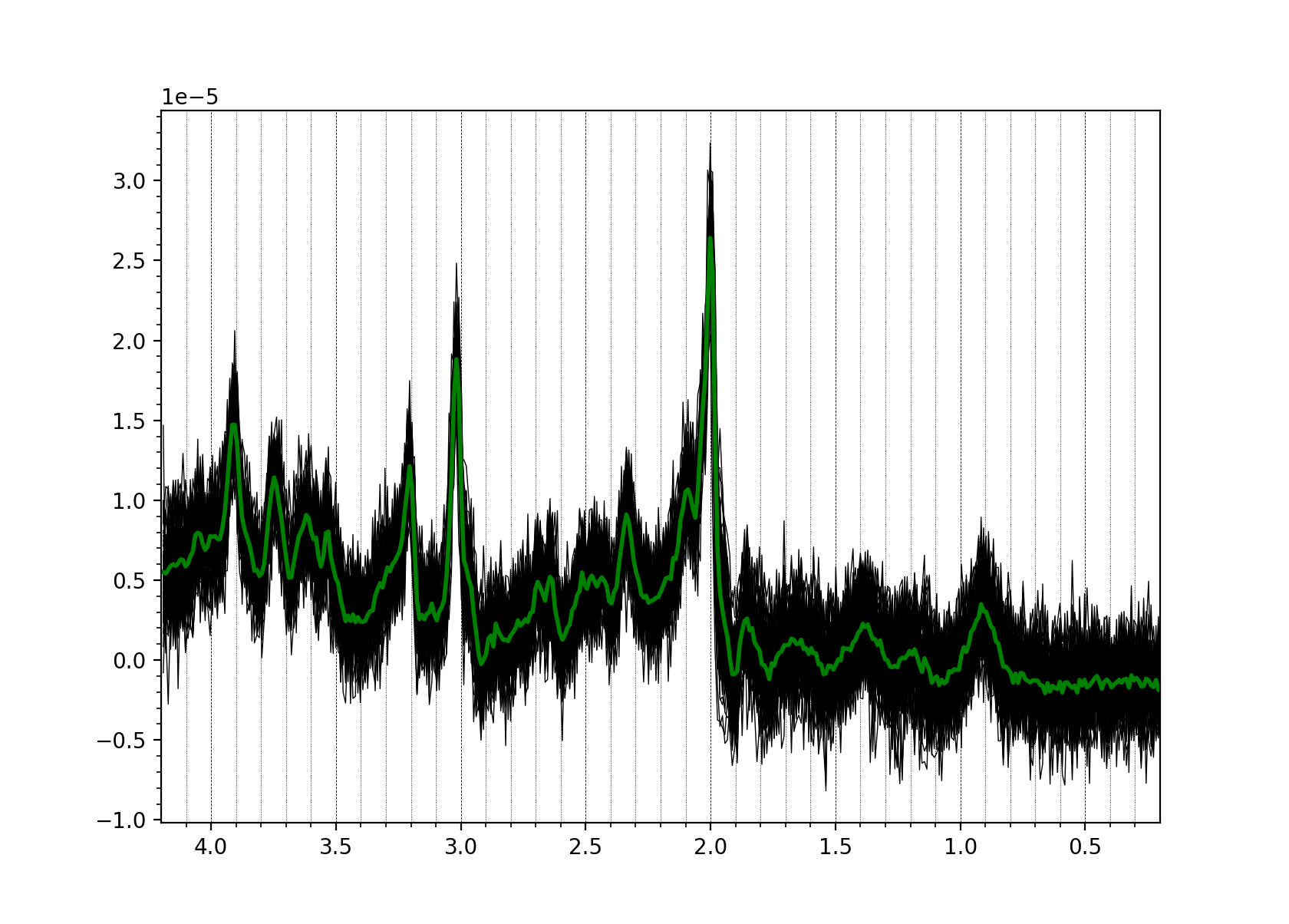
If you see a significantly different picture (no data, just noise, etc.) stop and investigate. See Troubleshooting.
Have a look at the Visualisation page for more information on mrs_tools vis.
2. Process your raw data
Some data requires pre-processing. Often MRSI data will have gone through appropriate pre-processing during reconstruction, if so skip to step 3. For unprocessed single-voxel (SVS) data, read on.
Use the fsl_mrs_proc commands to pre-process your raw data. fsl_mrs_proc contains routines for many common processing steps (e.g. coil combination, phase-frequency alignment, residual water removal). For example:
fsl_mrs_proc coilcombine --file my_metab_file.nii.gz --reference my_wref_file.nii.gz --output combined -r
fsl_mrs_proc align       --file combined.nii.gz --ppm 1.8 3.5                        --output aligned -r
fsl_mrs_proc average     --file aligned.nii.gz  --dim DIM_DYN                        --output avg -r
fsl_mrs_proc remove      --file avg.nii.gz                                           --output water_removed -r
fsl_mrs_proc phase       --file water_removed.nii.gz                                 --output metab -r
The -r requests a HTML report to be generated for each stage of the processing. The different HTML reports can be merged using:
merge_mrs_reports -d example_processing -o . *.html
If your data is unedited single voxel (SVS) try out the prepackaged processing pipeline fsl_mrs_preproc. You will need to identify the water suppressed and water unsuppressed files to pass to the script. For details on which water reference to use if you have multiple see the fsl_mrs_preproc section of the processing page.
fsl_mrs_preproc --output processed --data my_metab_file.nii.gz --reference my_wref_file.nii.gz --report
Have a look at the source code for fsl_mrs_preproc to see how you can construct your own python script using the processing modules. You can always prototype using Jupyter/IPython (see Demos)
3. Create Basis Spectra
If someone has provided you basis spectra, or you have an existing set in .BASIS format you can skip this section and go to step 4.
The fitting in FSL-MRS requires the user to provide basis spectra. Basis spectra are the simulated responses of the in vivo metabolites to the pulse sequence. FSL-MRS provides a simulator to create basis sets fsl_mrs_sim:
fsl_mrs_sim -b metabs.txt my_sequence_description.json
my_sequence_description.json contains a description of the sequence broken down into blocks of RF pulses and gradients. This must be created for each sequence manually once. metabs.txt contains a list of metabolites to simulate. Much more information on constructing a suitable sequence description JSON file can be found on the Basis Spectra Simulation page.
Have a quick check of your basis set using mrs_tools vis:
mrs_tools vis my_basis_spectra/
4. Tissue Segmentation
For FSL-MRS to produce accurate water scaled molarity or molality concentrations from the fitting results, it must be provided with estimates of the tissue (GM, WM, CSF) fractions in each voxel.
For this FSL-MRS provides the svs_segment or mrsi_segment commands for SVS and MRSI data respectively.:
svs_segment -t T1.nii.gz processed/metab.nii.gz
mrsi_segment -t T1.nii.gz mrsi_data.nii.gz
svs_segment creates a small JSON file segmentation.json which can be passed to the fitting routines. mrsi_segment creates NIfTI files of the fractional tissue volumes registered to the MRSI volume.
svs_segment and mrsi_segment both rely on fsl_anat to run FSL FAST tissue segmentation. If fsl_anat has already been run, then the -t T1.nii.gz option can be substituted with -a T1.anat.
Inputs to the segment commands are raw T1 images (i.e. not skull stripped) or the output of fsl_anat (FSL FAST segmentation must have been run).
5. Fitting
FSL-MRS provides two wrapper scripts for fitting: fsl_mrs (for SVS data) and fsl_mrsi (for MRSI data).
fsl_mrs  --data metab.nii.gz --basis my_basis_spectra --output example_svs  --h2o wref.nii.gz --tissue_frac segmentation.json --report

fsl_mrsi --data mrsi.nii.gz  --basis my_basis_spectra --output example_mrsi --h2o wref.nii.gz --mask mask.nii.gz --tissue_frac WM.nii.gz GM.nii.gz CSF.nii.gz --report
6. Visualise
HTML processing reports merged using merge_mrs_reports and fitting reports made using fsl_mrs and fsl_mrsi can be viewed in your browser.
For visualising MRSI data, fits, and fitting results, FSLeyes is recommended.
Demos
Demo Jupyter notebooks are provided alongside some sample data in the example_usage directory. These notebooks show an example processing pipeline implemented both on the command-line and in interactive python.
To access these clone the FSL-MRS GitLab with Git LFS installed.
You will need to have jupyter notebook installed:
conda install -c conda-forge notebook
Then start the notebook:
cd example_usage
jupyter-notebook
A window should open in your browser and you can select one of the four example notebooks.